My cuRFP library has virtually no overhead versus the standard cuBLAS library, just half the memory usage. The library has a PyTorch interface and is available on GitHub: https://github.com/andersx/curfp

Scaling beyond cuBLAS and PyTorch

Let’s say that you want to solve problem like Kernel Ridge Regression (KRR). This requires solving a matrix equation like

The bottleneck for scaling this is the Cholesky factorization of the kernel matrix $K$, which needs to fit entirely in GPU memory. cuRFP allows you to scale the problem size to twice the memory footprint compared to a dense matrix by storing the matrix in a packed format that reduces the memory usage from \(n^2\) to \(n(n+1)/2\).

I did some benchmarks of the Cholesky factorization with cuRFP versus CUDA’s built-in dense Cholesky factorization in cuSOLVER, and PyTorch’s wrapper around it.

I mostly use my RTX 5070 Ti GPU at home for hacking projects, and I am limited to 16 GB of memory. For bigger projects I’ve been using RunPod to rent H100s and H200s, but the price difference is significant, so I want to do as much as possible on my local GPU and fit on an H100 rather than an H200 if possible.

On an H200 with 141 GB of usable memory, here is how far I was able to get with each method:

In the end I was able to fit a 262K $\times$ 262K matrix on an H200 and run the Cholesky factorization with cuRFP, which is close to the largest possible dense matrix that can fit in 141 GB of GPU memory.

I found substantial memory overhead in the PyTorch implementation, I believe there is a matrix copy even when calling torch.linalg.cholesky(A, out=A) and trying to do it in-place. This is a bit surprising since the PyTorch docs say that the out parameter should allow in-place operation, but I wasn’t able to get it to work without the copy.

Calling cuSOLVER’s SPOTRF directly from CUDA gives much better memory usage compared to PyTorch, but still hits the limit at 185K because of the dense storage format.

The plot below shows the timings and memory usage for the three methods on a range of matrix sizes. There is slight additional overhead at small matrix sizes, this is negligible as the problem grows.

The Python interface for cuRFP is compatible with PyTorch, and most functions should be drop-in compatible with torch functions. Here’s a small example to solve a linear system with a symmetric positive definite matrix using cuRFP.

import torch
import curfp

n, k, nrhs = 4096, 128, 10

A = torch.randn(n, k, dtype=torch.float32, device="cuda") / k**0.5
C = torch.empty(n * (n + 1) // 2, dtype=torch.float32, device="cuda")
B = torch.randn(nrhs, n, dtype=torch.float32, device="cuda")

# Symmetric rank-k update: C = A @ A.T in RFP format
curfp.ssfrk(A, C)

# Regularize: C += I  (ensures positive definiteness)
curfp.add_to_diagonal(C, 1.0)

# Cholesky factorization in-place
curfp.spftrf(C)

# Solve (A @ A.T + I) @ X = B  in-place on B  (B is nrhs×n, rows are RHS)
curfp.spftrs(C, B)

The function names follow the name conventions from BLAS/LAPACK, so they might not always be totally obvious. I mirrored every function from BLAS/LAPACK that operates on symmetric matrices, so check out the docs https://github.com/andersx/curfp for a full list of functions.

I did add one quality of life upgrade from BLAS notation, and that is that matrix dimensions etc are autodetected, so mostly you just need to call a function with one or two arguments.

OK, so what is Rectangular Full Packed (RFP) format?

The RFP format is a neat trick to store an $n \times n$ symmetric matrix using only $n(n+1)/2$ floats — exactly half the storage of a full dense matrix. The trick is packing the memory in such a way that standard BLAS/LAPACK operations can be applied directly to the packed submatrices by adjusting stride and dimension parameters. Matrix operations on RFP matrices require the same FLOPs as their dense counterparts, so there is no computational penalty, only the minuscule overhead of 2–3 extra BLAS calls.

I think this is the main reference if you’d like to read more about RFP format from the original inventors: https://www.netlib.org/lapack/lawnspdf/lawn199.pdf

Let’s say we have a $5 \times 5$ symmetric matrix stored with the upper triangle convention. We will use red, blue, and green to label the three blocks consistently throughout this post. For odd $n$, the RFP layout splits the matrix into two triangular diagonal blocks and one rectangular off-diagonal block:

Here the red and blue blocks are symmetric diagonal blocks, and the green block is a rectangular off-diagonal block.

We can visualize this in RFP format:

The top $3 \times 3$ part contains the two triangular diagonal blocks folded together, while the bottom $2 \times 3$ part is the rectangular green coupling block.

The packing is slightly different for even $n$ (the fold point shifts by one row). Combined with the upper/lower triangle convention and an optional transposition of the whole packed rectangle (transr), there are 8 RFP layout variants in total. cuRFP handles all of them through a single parameter struct so the calling code never has to think about it.

Example 1: Symmetric rank-k update in RFP format: SFRK

This is probably the simplest example to show how RFP is implemented in practice. Let’s say you want to compute a symmetric matrix product $A = X X^\top$. If you do this with BLAS you have a few options:

• GEMM: Standard matrix-matrix multiplication which results in a full $n \times n$ matrix.
• SYRK: Better option — only computes the upper or lower triangle of the result and uses half the FLOPs, but still requires $n^2$ memory.
• SFRK: Computes the result directly in RFP format, giving the same FLOPs as SYRK but only half the memory. Available in MKL and Apple Accelerate; cuRFP brings it to CUDA.

To see why this works, split $X$ into the same row blocks as the RFP matrix:

where for the $5 \times 5$ example above, $X_1$ has 3 rows and $X_2$ has 2 rows. Then

This maps directly to three BLAS calls:

So instead of forming one large dense matrix, SFRK computes two symmetric rank-$k$ updates for the diagonal blocks and one ordinary matrix multiply for the rectangular off-diagonal block. The RFP layout ensures the triangular diagonal blocks are stored such that SYRK can write results directly to the correct memory locations when stride and dimension parameters are set correctly — so SFRK is really just three BLAS calls.

In my code this is roughly how it looks (there is a bunch of code to determine the correct block sizes and offsets for the different RFP layouts, but the core of the SFRK operation is these three calls):

    /* symmetric rank-k update on red diagonal block */
    cublasSsyrk(cb, p.fill1, opA,
        p.dim1, k, alpha, A1, lda, beta, C + p.off1, p.ldc);

    /* sgemm on green off-diagonal block */
    cublasSgemm(cb, opA, opAt,
        p.gemm_m, p.gemm_n, k,
        alpha, Ag1, lda, Ag2, lda, beta, C + p.offg, p.ldc);

    /* symmetric rank-k update on blue diagonal block */
    cublasSsyrk(cb, p.fill2, opA,
        p.dim2, k, alpha, A2, lda, beta, C + p.off2, p.ldc);

This has the same FLOPs as a normal symmetric matrix multiplication done with a big SYRK call, but only uses half the memory. The only minor overhead comes from the extra logic to determine the correct parameters, and the additional overhead for the two extra BLAS calls, but in practice this is negligible compared to the memory savings and the fact that you can now fit much larger matrices on the GPU.

I like this approach a lot, since it will continue to be very performant in the future, as any improvements to cuBLAS will directly be used in cuRFP.

Below are the timings for cuRFP’s SFRK versus a dense SYRK in cuBLAS, and PyTorch’s mm (which computes the full dense product) on an H200 GPU. PyTorch has no direct counterpart to SYRK so I felt like the user might resort to using torch.mm() here.

The timings for cuRFP are very close to cuBLAS SYRK, so the three cuBLAS calls don’t seem to have any detrimental effect at larger problem sizes. Both cuBLAS and PyTorch only scale to n = 185K on an H200 as expected. PyTorch is 2x slower since it computes both the upper and lower triangle via cuBLAS GEMM.

Example 2: Cholesky factorization

Now we are getting to the meat of it. I really wanted to do this to be able to factorize larger matrices for kernel-ridge regression and Gaussian-process regression on GPUs.

The RFP approach can also be applied to Cholesky factorization, which is the main bottleneck for training and optimizing kernel-based methods.

The Cholesky factorization of a symmetric positive definite matrix $A$ is given by $A = L L^\top$, where $L$ is a lower triangular matrix.

We can apply the same block-decomposition trick. Splitting $A$ into the same red upper-left, blue lower-right, and green off-diagonal blocks, the factorization becomes:

where ${\color{red}L_{11}}$ is the lower-triangular Cholesky factor of the red diagonal block, ${\color{blue}L_{22}}$ is the lower-triangular factor of the blue diagonal block, and ${\color{green}L_{21}}$ is the dense green off-diagonal block of $L$.

Multiplying the two block matrices on the right and matching against $A$ gives three equations:

Each of these maps directly to one BLAS or cuSOLVER call, in this exact order:

The RFP layout makes sure that the three blocks can be indexed contiguously with a bit of logic to determine the offsets and strides.

In the end the SPFTRF routine for Cholesky factorization in cuRFP looks something like this:

    /* Step 1: Cholesky of red diagonal block */
    cusolverDnSpotrf(cs, p.fill1, p.dim1,
        C + p.off1, p.ldc, work, lwork, devInfo);

    /* Step 2: triangular solve for green off-diagonal block */
    cublasStrsm(cb, CUBLAS_SIDE_RIGHT, p.fill1, CUBLAS_OP_T, CUBLAS_DIAG_NON_UNIT,
        p.gemm_m, p.dim1, &one, C + p.off1, p.ldc, C + p.offg, p.ldc);

    /* Step 3: rank-k update on blue diagonal block */
    cublasSsyrk(cb, p.fill2, CUBLAS_OP_N,
        p.dim2, p.dim1, &m_one, C + p.offg, p.ldc, &one, C + p.off2, p.ldc);

    /* Step 4: Cholesky of updated blue diagonal block */
    cusolverDnSpotrf(cs, p.fill2, p.dim2,
        C + p.off2, p.ldc, work, lwork, devInfo);

Here are the timings I got from running cuRFP on a H200 on my RunPod: Again, there is no real timing difference between pytorch, directly calling cuBLAS or cuRFP. But curfp can go further.

To actually solve a linear system with the Cholesky factorization, you can use the SPFTRS routine in cuRFP, which performs a triangular solve using the Cholesky factor in RFP format. See the earlier code snippet for an example of how to use it.

The scaling result is similar to the two previous examples, with cuRFP scaling to larger matrices than cuBLAS and PyTorch with no overhead.

Installation

I plan to make this a pip package, but for now I am lacking a way to do CI testing with GPU support, so for now you will have to do something like:

git clone https://github.com/andersx/curfp.git
uv pip install -e curfp

Requirements are pretty mild: A working PyTorch installation with CUDA 12.8 or later.

Supported operations

cuRFP implements the following functions, all operating directly on the packed RFP buffer with no pack/unpack step:

All functions are available in both single (s prefix) and double (d prefix) precision, e.g. ssfrk / dsfrk, spftrf / dpftrf, etc.

All functions support all 8 RFP storage variants (transr × uplo × n parity) and accept an optional CUDA stream for asynchronous execution.

Conclusion

The library is in a good working state, and is available at https://github.com/andersx/curfp under the MIT license. I would greatly appreciate any PRs or open issues.

I am still figuring out a sustainable way to do the GPU-based CI testing and release a pip package, but in the meantime try it out and save yourself memory!

– Anders

I did some work back in my post doc days with approximate kernels that I never published, so I am writing a few blog posts to share the work. I’m starting with a practical intro to GPR+UQ and then I will move on to approximate kernels.

In this first part, I will just cover the basic GPR equations and how to implement them. The next posts will cover:

• GPR+UQ with derivatives (e.g. for molecular forces)
• Practical examples of GPR+UQ in chemistry
• UQ for approximate kernels

Introductory notes and notation

In textbooks, the predictive mean and variance are usually written as

and

where the first equation is very analogous (basically identical) to kernel-ridge regression (KRR).

Here I use a hat, $\hat{\cdot}$, to denote predicted quantities, and an asterisk, $*$, to denote a test point. $\mathbf{x}$ is the feature vector or representation for a training/test point.

In this notation:

• $\mathbf{K}$ is the $n \times n$ kernel matrix over the training data, with entries \(K_{ij} = \mathpzc{k}(\mathbf{x}_i, \mathbf{x}_j),\)
• $\mathbf{k}_*$ is the $n \times 1$ covariance vector between the test point $\mathbf{x}_*$ and all training points, \(\mathbf{k}_* = \begin{bmatrix} \mathpzc{k}(\mathbf{x}_1, \mathbf{x}_*) \\ \vdots \\ \mathpzc{k}(\mathbf{x}_n, \mathbf{x}_*) \end{bmatrix}.\)

These equations are correct, but they are slightly misleading from an implementation point of view. For example, you would never explicitly compute the inverse of $\left(\mathbf{K} + \lambda \mathbf{I}\right)^{-1}$. Plus a few other differences that we’ll get to later/

Training the model

Our task here is to solve for the regression coefficients $\alpha$:

In practice, you wwill never form the inverse explicitly. Instead, the most efficient approach is to do a Cholesky factorization the regularized kernel matrix and solve linear systems:

with

where $L$ is lower triangular (L is for lower).

This is both more numerically stable and more efficient than forming the inverse explicitly. It also avoids storing the inverse matrix in memory. Instead of storing an $n \times n$ dense inverse, you only keep the lower-triangular Cholesky factor, which requires $\tfrac{n(n+1)}{2}$ entries if you work with packed storage matrices.

In LAPACK, this is typically done with dpotrf. In Python, this corresponds to numpy.linalg.cholesky() or scipy.linalg.cho_factor().

Using the Cholesky factorization, this is equivalent to solving two triangular systems:

followed by

In LAPACK, this is usually handled by dpotrs which actually does both solves in one go. In SciPy, the corresponding interface is scipy.linalg.cho_solve().

Heres a very minimal example using qmllib in Python:

import numpy as np
from scipy.linalg import cho_factor, cho_solve
from qmllib.kernels import gaussian_kernel 

# X_train = test set representation matrix, ell = lenght scalce of kernel (l)
# K is the n_train x n_train kernel matrix over the training data
K = gaussian_kernel(X_train, X_train, ell)

# Add regularization / observation noise to the diagonal
K[np.diag_indices_from(K)] += lambda_

# Cholesky factorization - save this one for later
L, lower = cho_factor(K, lower=True)

# Solve (K + lambda I) alpha = y
alphas = cho_solve((L, lower), y)

A useful shortcut for the training residual

Heres a small trick I find very useful in practice: After training, you often want to compute the training residuals, which are the differences between the training labels and the predictions on the training set.

Looking at the equations you might think you would need the same kernel matrix as you just used to to solve the regression coefficients, but actually you can compute the training residual without that big kernel.

Lets define the residual error (difference between true labels and predictions) as:

Since the predictions on the training set are

we have

Now use the fact that the fitted coefficients satisfy exactly that

Substituting this into the residual expression gives

and, since the $\mathbf{K}\alpha$ terms cancel out, therefore

Once you have computed $\alpha$, you can discard $\mathbf{K}$ and get the training residual for free.

Predicting at test time

Ok, now we are ready to do inference on new test points.

For a test point $\mathbf{x}_*$, first compute the covariance vector

The predictive mean is

Once $\alpha$ has been computed during training, this is just a dot product between the test covariance vector and the stored coefficients.

Predictive variance

The textbook formula is

Again, we do not form the inverse explicitly. Instead, we use the same Cholesky factor $L$ and solve

Then

This works because

-Ok, but we’re not done yet! Just implemnenting the equation above will likely not give you what you are looking for

Unit scale of the predictive variance?!

You might notice this: if the kernel is unitless, then the predictive uncertainty is also unitless, which is a bit totally weird. In contrast, the predictive mean is in the same units as the training labels, and the units of the training labels seem to get absorbed into alpha.

In fact, you can see that no matter what labels you put in your $\mathbf{y}$ vector, the predictive variance formula seems to give the same variance. But we’d expect that you’d get a 1000 times larger variance if you trained on labels in millimeter instead of meter, for example.

This is because commonly, the kernel in GPR is defined to contain the signal variance $\sigma_f^2$ as a multiplicative factor, e.g. for the scaled RBF kernel:

GPR expects the signal variance factor, whereas in e.g. KRR, the kernel is defined without it.

So, if you just want to work with a “normal”, unitless kernel, for example the Gaussian: $\mathpzc{k}^{\text{unitless}}(\mathbf{x}, \mathbf{x}’) = \exp\left(-\frac{|\mathbf{x} - \mathbf{x}’|^2}{2l^2}\right)$, then the equations change slightly. The predictive mean is still \(\hat{y}_* = \mathbf{k}_*^\top \alpha\), since the “missing” scaling is absorbed into $\alpha$ during training.

However, the predictive variance is missing the signal variance factor, so we need to add it back in explicitly, and the predictive variance becomes:

To further simplify things for the unitless Gaussian kernel, the self-kernel \(\mathpzc{k}^{\text{unitless}}\left( \mathbf{x}_*, \mathbf{x}_*\right)\) is always 1, so the predictive variance simplifies to a very simple form:

Ok, so what is the value of $\sigma_f^2$? In principle, it’s a hyperparameter that needs to be fitted, for example to a validation set to calibrate the predictive uncertainty. In practice you can use the maximum likelihood estimate of $\sigma_f^2$ from the training data, which is given by the average product of the training labels and the regression coefficients:

Putting it all together, here is a complete example of the variance estimation at test time:

import numpy as np
from scipy.linalg import solve_triangular
from qmllib.kernels import gaussian_kernel 

# --- Prediction at a test point ---
# K_star is the n_train x n_test covariance vector between x_* and training points
K_star = gaussian_kernel(X_train, X_test, ell)

# Predictive mean for test points
y_pred = K_star.T @ alphas

# MLE estimate of signal variance
sigma_f_sq = y @ alphas / len(y)

# Predictive variance for test points
v = solve_triangular(L, K_star, lower=True)
var_pred = sigma_f_sq * (np.ones(n_test) - np.sum(v**2, axis=0))

In my next blogpost, I will show how to do variance calculation with kernel-derivatives for molecular energy and forces with a few practical examples.

-Anders

Mostly it has been running flawlessly, with the major problems actually being with Nvidia drivers. But not this time…

Since the last update to the Battle.net app, I had a lot of trouble getting it to run on my Ubuntu 24.04. Funny thing is that StarCraft II would run fine, but the Battle.net app would not allow logging in. And eventually StarCraft II got patched requiring me to use the Battle.net app to launch it, which I could not do.

Turns out it was an outdated Wine version that was the problem. So here is how I got it working again in early 2026 on Ubuntu 24.04 LTS.

Step 1: Install a custom Wine version using ProtonUp-Qt

I was having a lot of problems logging in to the Battle.net app until I switched to a custom Wine version. For this I found that I needed to install a different runner than the default wine runner that ships with Lutris.

This step is a prerequisite for the next step.

Someone conveniently made a manager called ProtonUp-Qt that can install custom Wine/Proton versions for Lutris and Steam. This manager is managed through yet another package manager Flatpak.

# Install protonup-qt via flatpak
flatpak install flathub net.davidotek.pupgui2

# Run protonup-qt with flatpak
flatpak run net.davidotek.pupgui2

In ProtonUp-Qt, select Lutris (/path/to/lutris) drop down menu Install For, and then select Add version -> Compatibility tool: == Wine Tgk (Vale Wine Bleeding Edge) and Version: == 20028xxxx whatever the top of the list number in the list is (at the time of writing it was 10.0.28.0432).

Then press the Install button. After a while you should see something like: wine-tkg-valve-exp-bleeding-experimenta.bleeding.edge.10.0.28.0432.20251205 in the list of install tools (was the latest version that I am using at the time of writing).

Step 2: Installing Lutris

The recommended way to install Lutris on Ubuntu is via .deb files off of Github. Unfortunately, there is no PPA available for ubuntu 24.04 LTS at the moment that I could find. I think it exists for 22.04, so you can probably use the PPA if you are still on 22.04.

So go to https://github.com/lutris/lutris/releases and download the latest .deb file.

Now, install some dependencies for Lutris and Wine to function:

sudo dpkg --add-architecture i386
sudo apt update
sudo apt install libgl1:i386 libgl1-mesa-dri:i386 libgnutls30:i386 mesa-vulkan-drivers:i386 python3-protobuf protobuf-compiler wine

You can use apt to install the .deb file, which will automatically resolve the dependencies for the .deb file:

sudo apt update
sudo apt install ~/Downloads/lutris_0.5.18_all.deb  # Note the absolute path 

Step 2.5: Setting up Lutris

Now start Lutris from your application menu or by running lutris -d in a terminal. A bunch of addons will be installed the first time you run it (lower left corner). Wait for these to finish.

If you see any missing dependencies warnings, install the missing dependencies (I believe I have most of them installed from the previous step, though).

Important:

• Make sure you have the latest Wine version installed via ProtonUp-Qt as described in Step 1
• DO THIS BEFORE PROCEEDING TO STEP 3: Now, click the Wine gear icon in the bottom left in lutris and click on the dropdown menu for Wine version and select the bleeding edge version you installed with ProtonUp-Qt. This makes sure that Lutris uses the correct Wine version when installing Battle.net.

Ok, with Lutris set up and the correct Wine version selected, we can now proceed to install Battle.net.

Step 3: Installing Battle.net via Lutris

Now go to the Lutris page for Battle.net app: https://lutris.net/games/battlenet/ Press the “Install” button, and Lutris should open up and guide you through the installation process.

• DO NOT INSTALL MONO If prompted to install Mono, press cancel (it can freeze the process).
• You can also download the execuable from e.g https://www.blizzard.com/en-us/apps/battle.net/desktop and point Lutris to that file during installation, in case the automatic install script does not work. Both worked for me this time, but I’ve had problems with the automated downloader in the past.

Quick command to download the Battle.net installer:

wget "https://www.battle.net/download/getInstallerForGame?os=win&version=LIVE&gameProgram=BATTLENET_APP" -O Battle.net-Setup.exe

This can take some times (a few minutes) before you’ll get to the the dialog boxes to log in to your Battle.net account etc. Once you have logged in exit the Battle.net app from the menu in the top left corner.

Step 4: Running Battle.net

Start Lutris again from the terminal lutris -d, and double click on Battle.net in your library to start it up. Then you can install your games as usual.

I tried this on two different Ubuntu 24.04 LTS machines, one with an Nvidia GPU and one with an Intex iGPU and was successful on both instances. I tested StarCraft II on both and they worked, I am not sure about other games.

– Anders

I found a forum post that mentioned a similar problem and that disabling power saving for the WLAN interface could help.

See also this Raspberry Pi StackExchange thread.

Check the status of power saving with the command:

iw dev wlan0 get power_save

What I did was to create a udev rule that permanently disables power saving for the WLAN interface. Might not be the best option for power saving, but if you want to rely on SSH access, etc. and you are hardwired on power anyway its probably fine.

Create a file /etc/udev/rules.d/70-wifi-powersave.rules with the following content:

ACTION=="add", SUBSYSTEM=="net", KERNEL=="wlan*", RUN+="/sbin/iw dev %k set power_save off"

Reboot.

Check again with:

iw dev wlan0 get power_save

It should now say Power save: off.

– Anders

I live close to Copenhagen Airport, and I care about the local air quality. The pollution in this area particularly due to particle emissions from aircrafts and woodburners. This project is my attempt to monitor the environment on Amager, and to raise awarenss.

According to the Danish Ministry of the Environment, an estimated 4,000 Danes die prematurely every year due to air pollution–that’s more than 10 people every day.

Ny rapport: Bedre luftkvalitet medfører 380 færre for tidlige dødsfald pga. luftforurening (Miljøministeriet, marts 2025)

I am working on open-source hardware and software to make this project possible. The goal is to create a low-cost air quality monitoring system that can report from multiple locations, and to make the data available to the public.

Right now, I am sharing the data from my prototype (see below), but I am also working on a more robust version that will be deployed outdoors.

I’ve designed a PCB that is being manufactured, and I need to do more testing before I can deploy more measureing stations.

What is PM2.5?

I’m focusing on a specific type of air pollution: PM2.5. PM2.5 refers to fine particulate matter that is 2.5 micrometers or smaller in diameter. These particles are small enough to penetrate deep into your lungs and even enter your bloodstream.

The reason that I am focusing on PM2.5 is a good measure of particle pollution, and it is also realitvely easy to measure.

What is measured?

The PM2.5 levels are measured in micrograms per cubic meter of air (µg/m³) . The World Health Organization (WHO) recommends that PM2.5 levels should not exceed 5 µg/m³ as an annual mean, and 10 µg/m³ as a 24-hour mean.

As you can probably see from the plot above, the levels in my area are often much higher than this.

During the winter months, when the air quality is often poor due to woodburning in private households. Woodburners are the single largest source of PM2.5 emissions in Denmark, and they are responsible for about 43% of the total PM2.5 emissions in the country according the Danish Ministry of the Environment.

In the summer, the levels are mostly affected by emmisions from the airport, and will depend heavily on the wind direction.

One goal of this project is to collect the data do document this and estimate the health effects.

What hardware am I using?

I’m currently using a PMS5003 sensor, which is a low-cost laser-based sensor that can measure PM1.0, PM2.5, and PM10 levels.

If you are interested you can read a scientific review of the PMS5003 sensor here:

Nam H. Nguyen, Huy X. Nguyen, Thuan T. B. Le, Chinh D. Vu, published by Open Journal of Air Pollution, Vol.10 No.1, 2021.

For practical purposes the accuracy is about ±10% for PM2.5, which is more than sufficient for this project - simply to determine whether the air quality is mostly good or bad.

How It Works

This is a custom solution built with open-source tools and low-cost hardware:

• I’m using an ESP32 microcontroller connected to the PMS5003 particle sensor.
  • The PMS5003 sensor continuously measures particle levels and sends the data to the ESP32.
• The ESP32 pushes data to a bucket on InfluxDB Cloud every few minutes.
• A simplecron job on my Raspberry Pi pulls this data periodically, processes it, and uploads it to a public GitHub repository.
• This blog then loads the latest data from that github repo and serves it in the plot above.

Future Plans

My plan is to monitor the air quality from several locations on Amager, and to make the data available to the public.

To make this possible, I’m currently working on a custom PCB to integrate everything.

• It will include the PMS5003, an ESP32, and support for a small LCD display.
• I’m also designing a 3D-printed enclosure to make the sensor weatherproof and mountable outdoors.
• Here’s a preview of the prototype being manufactured:

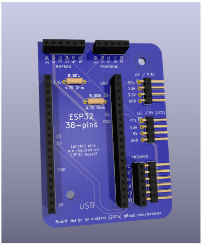
I designed the board in KiCAD, and it’s currently being fabricated by PCBWay.

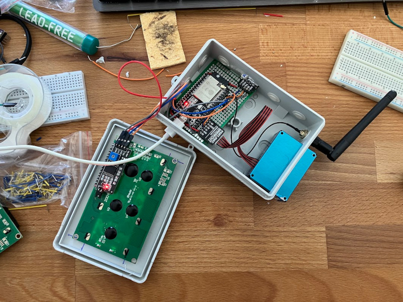
Photos of the Current Setup

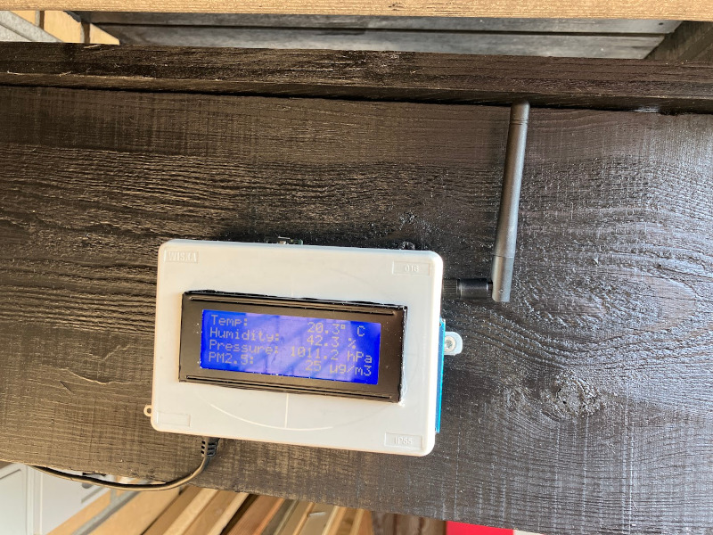
Here’s the current test setup, mounted under my soffit:

And here’s the final version enclosed and deployed:

– Anders

Jeg bruger i denne guide en Unifi UCG-Ultra med UniFi OS version 4.1.13 og Unifi Network version 9.0.114. Routeren er tilsluttet direkte fra sit WAN-stik til en LAN-port i fiberboksen fra TDC.

Alt konfigureres direkte i UniFi Network-appen, og det var ikke nødvendigt at genstarte routeren undervejs — heller ikke ved skiftet fra min tidligere udbyder (Hiper) til NetNørden.

Du kan også trykke her for at se min guide til opsætning af IPv6 hos Hiper.

Opsætning af WAN med IPv4 og IPv6

1. Log ind på din UniFi Controller og gå til Settings > Internet

2. Vælg Primary (WAN1) og klik på Manual

3. VLAN ID skal være slået fra. (De fleste udbydere kræver VLAN ID = 101, men NetNørden gør ikke.)

4. Din IPv4 Configuration burde virke med indstillingen fra Auto, intet at ændre her.
5. Under IPv6 Configuration, vælg:
   • IPv6 Connection: DHCPv6
   • Prefix Delegation Size: 48 (NetNørden bruger /48)
     • Auto - NetNørden tildeler dynamisk prefix /56 (Updated December 2025)
   • DNS Servers: Auto
6. Klik på Apply Changes og vent — din router bør få tildelt en offentlig IPv6-adresse med det samme. Jeg skulle hverken genstarte eller unplugge routeren, før det virkede - fantastisk!

Opsætning af LAN med IPv4 og IPv6

1. Gå til Settings > Networks, og vælg dit LAN-netværk i listen (typisk kaldet Default)
2. IPv4-opsætningen burde virke med Auto
3. Gå til IPv6, vælg Prefix Delegation, og lad resten af indstillingerne være uændrede
   • Advanced kan bare stilles til Auto, så burde det køre fint med SLAAC på dit LAN.

Det burde være alt der skal til!

Test opsætningen

• Check at din router har fået tildelt en offentlig WAN IPv6 adresse på forsiden af Unifi Network. Hvis du har fast IP burde du kunne se den IPv4 og IPv6 du har fået tildelt i din velkomst email.

• Check at din computer har fået en IPv6 adresse f.eks. nmcli device show | grep IP6 i terminalen:

$ nmcli device show | grep IP6
IP6.ADDRESS[1]:                         ****:****:****:****:***:****:****:****/64
IP6.ADDRESS[2]:                         ****:****:****:****:****:****:****:****/64
IP6.ADDRESS[3]:                         ****::****:****:****:****/64
IP6.GATEWAY:                            ****::****:****:****:****
IP6.ROUTE[1]:                           dst = ****::/64, nh = ::, mt = 1024
IP6.ROUTE[2]:                           dst = ****:****:****:****::/64, nh = ::, mt = 100
IP6.ROUTE[3]:                           dst = ::/0, nh = ****::****:****:****:****, mt = 100
IP6.DNS[1]:                             ****:****:****:****::1
IP6.GATEWAY:                            --
IP6.GATEWAY:                            --
IP6.ADDRESS[1]:                         ::1/128
IP6.GATEWAY:                            --
IP6.ROUTE[1]:                           dst = ::1/128, nh = ::, mt = 256

For at teste at IPv6 virker korrekt kan du f.eks. bruge sikkerpånettet.dk/connection/.

Glædelig IPv6!

I wanted a simple but robust setup to continuously log humidity (and temperature) data from an ESP32-based sensor, store it in a CSV file, and push it to GitHub where it could be visualized and accessed easily.

The data comes from a sensor connected to an ESP32 microcontroller. Live output is served via JSON/requests from webserver running on the ESP32. My Raspberry Pi collects this data every minutes via a cron job. Every 1 hour, my bot andersx-bot automatically pushes it to a GitHub repository: 👉 View the CSV on GitHub

This keeps things super lightweight and easy to scrape.

Rather than generating static plots, this page dynamically fetches the latest CSV data from GitHub and visualizes it using Plotly.js — entirely in your browser.

How it works

• Hardware: ESP32 with a humidity sensor - served data in JSON format over HTTP
• Collector: Raspberry Pi pulls data every 5 minuts via a cron job
• Uploader: GitHub bot commits+pushes to the CSV every few minutes
• Frontend: JavaScript fetches and visualizes the data live with Plotly on this page

This setup ensures the chart is always up-to-date without needing server-side rendering or plot regeneration, and cleanly separates the data collection from the visualization.

For this example, I am using the UCG-Ultra running UniFi OS version 4.1.13 with Network version 9.0.114. The Ubiquiti router should be connected directly to the fiber ONT box.

1. Configure the Internet Connection (WAN)

These steps will enable your WAN connection and set up IPv6:

1. Navigate to Settings:
   Click the gear icon and select Internet.

2. Enable VLAN Tagging:
   Hiper (and most other Nuuday ISPs) use VLAN tagging on the WAN interface. Check the VLAN tagging option and enter 101 as the VLAN ID.

3. Set DHCP for Both IPv4 and IPv6:
   • Ensure both IPv4 and IPv6 are set to DHCP.
   • For IPv6, set the Prefix Delegation Size to 48.
4. Reference Screenshot:
   

2. Configure IPv6 on the LAN

Follow these steps to enable IPv6 on your LAN:

1. Access Network Settings:
   Click the gear icon, then go to Networks. Select your network from the list (the default name is “Default”).

2. Set Up IPv6:
   • Click the IPv6 tab.
   • Change the Interface Type to Prefix Delegation.
3. Reference Screenshot:
   

3. Verify IPv6 Functionality

Ensure that IPv6 is working properly:

1. Check the WAN Side:
   Open the landing page of the Network Controller application. You should see details similar to the screenshot below:

   

2. Test LAN Devices:
   Devices on your LAN should now receive an IPv6 address and be able to access the internet. Verify by visiting Test IPv6—a perfect configuration will yield a 10/10 score.

   

Final Words

• Feedback: If you find any errors or have suggestions for improvements, feel free to open an issue or submit a pull request.
• Support: I no longer use Hiper myself, but I will do my best to assist if you encounter any problems.

The purpose here is to fire up an EC2 compute server, run a program, and save the output from that program on our local compute cluster at the university.

Basically, you just need to add a line to /etc/fstab and save the instance as an image (that’s what I did).

🧰 What you need:

• An Amazon EC2 instance with sshfs installed.
• A user with SSH keys properly set up to access the remote system (the SSH keys must not require a passphrase).

Let’s say your remote server has a folder named remote_folder
And your EC2 instance has a local mount point at local_folder.

Amazon EC2 Ubuntu instances typically use the ubuntu user, so the example assumes that.

Here’s the line to add to /etc/fstab (all on one line):

sshfs#ubuntu@remoteserver:/home/ubuntu/remote_folder/ /home/ubuntu/local_folder/ fuse user,delay_connect,_netdev,reconnect,uid=1000,gid=1000,IdentityFile=/home/ubuntu/.ssh/id_rsa,idmap=user,allow_other,workaround=rename 0 0

Notes:

• IdentityFile should point to your private SSH key.
• _netdev ensures the mount happens after the network is available.
• reconnect attempts automatic reconnection.
• delay_connect and workaround=rename are often needed to avoid weird mount issues (especially on boot).

⚠️ Don’t forget the trailing slashes (/) on both folder paths — it won’t work without them (speaking from bitter experience!).

🔄 Optional: Prevent SSH disconnects

To avoid idle SSH sessions timing out, add this line to your /etc/ssh/ssh_config:

ServerAliveInterval 5

This sends a keep-alive signal every 5 seconds.

That’s it!
Simple, minimal, and works well when you’re spinning up EC2 machines to crunch data and dump output to a shared server.